Objects in this document may appear out of sequence if not viewed with Internet Explorer

ORMSware^TM Suite is a product of Ushar Enterprises Inc, Littleton, Colorado, USA

Problem 5: Fleet Flow

A dedicated truck services company wants a descriptive (what-if) model for sizing a dedicated fleet for a customer based on recurring weekly delivery requirements. The focus during initial phase of the analysis is investment and operational cost consequences of any given fleet size. The what-if model is to be used as a response object to NMOD's Optimization Module to find fleet size with the lowest total costs.

Notes

• When a proposed fleet size is insufficient to meet customer’s shipping demands for a given weekday, loads that cannot be handled with trucks in the fleet are outsourced. When too many truckloads have to be outsourced, chances are the company can increase financial performance by increasing fleet size. 

• When available trucks in the fleet exceed demand on any given day, some trucks in the fleet are left idle. When too many trucks are idle, chances are the company can increase financial performance by decreasing fleet size.

• Proper formulation of this problem is a normative model which prescribes optimal fleet size for a dedicated operation. But, the purpose of this example is to show how to build a descriptive model of a situation to facilitate what-if analysis and then use the descriptive model for Fibonacci (response surface) search to prescribe optimal fleet size.

• We will also use this example to explain how a more comprehensive model can be built with due consideration of other operational matters in choosing appropriate fleet size. Such complex issues may not lend themselves to easy normative formulation, requiring descriptive models such as this one to find optimal solutions using response surface search.

• The label fleet trucks is used here to distinguish trucks in the fleet from contractor trucks carrying outsourced loads.

The problem is modeled here as a closed system with fixed resources and deterministic, totally predictable, recurring weekly demands for the resources, since the fleet will be dedicated to a customer. The resources are fleet trucks and demands are truckloads to be shipped to various destinations. The loads transition fleet trucks from available or idle status to busy status for a certain period of time before returning them to available status.

When a fleet truck is assigned to deliver a load, it becomes unavailable to satisfy other demands for a certain period of time. The length of time that truck will be unavailable depends on how long it has to travel to deliver a load and return to base.

In this example, we have classified demands by route durations/route zones. Zones were determined in terms of route durations of one, two, and three days. It will be obvious to the reader that this model can be scaled to refine and extend zone classifications to a minimum of any fraction of a day to a maximum of any multiple of the minimum duration. 

From recurring weekly shipping demands projected by the customer, demands for each day of the week were grouped in terms of the number of days they cause a truck to be unavailable (i.e. in terms of route duration/route zones), as shown in the image of the Excel table above.

On any given day when available fleet trucks are insufficient to handle all of that day's demands, excess demands are outsourced; if there is insufficient demand to assign all available fleet trucks, the unassigned trucks go into idle state till the next time period, which is the next day in this formulation.

• On the margin, outsourcing is more expensive than satisfying demands with trucks in the dedicated fleet. (Otherwise, it might make more sense to outsource the whole operation.)

• Because outsourcing is more expensive than using fleet trucks, one-day route deficits should be outsourced first, then two-day routes and three-day routes, in that order. This may be a myopic policy, since it is quite possible that in some cases such an outsourcing policy could cause costlier truck assignments in subsequent days. But, the purpose of this example is merely to demonstrate how problems are modeled using ORMSware's NMOD, not to research the best assignment policy.

Formulation of this problem is more easily understood through its ORMSware network diagram and its supplemental data files. Click the links below to open these files in separate windows for reference while reading the rest of this document.

VSD file: Image of Visio network file describing the model.
NET file: Contains expanded logic, if any, underneath each node and arc.
ADD file: If link exists, contains procedures supplied by analyst to link with NET file.
PGM file: If link exists, contains model execution control statements supplied by analyst.
Results: Preview of results of this model.

Following section describes the model:

• Total demand on any given day is the sum of truckloads to be shipped that day to all route zones.

• Total supply of fleet trucks in any given time period (day) is the sum of all fleet trucks that have returned in time to meet that time period's (day's) demand plus idle trucks, if any, left over from previous time period (day).

• Idle trucks on any given day are those fleet trucks that could not be assigned loads on that day due to insufficient total demand on that day.

• Outsourced truckloads on any given day are loads that cannot not be assigned to fleet trucks, because not enough fleet trucks are available to meet that day's total demand.

• Since demand pattern is exactly the same every week and truckloads that cannot be hauled by fleet trucks are always outsourced, truck assignment and truck flow are always balanced, and exactly the same, every week.

The model starts execution at the green Start node, viz. n[1]Initializations. The node happens to be [Visio-assigned] object number 1 in this case, indicated as [1] in the line above the node name. Analysts typically model the middle parts of a model first before dealing with the Start node, so Start nodes often have object numbers other than 1.

The content of n[1]Initializations can be viewed by locating it in the NET file. Content of n[1]Initializations is large, but consists mostly of simple assignment statements for initializing several variables, except for the SignalTarget procedure property, which we will cover in the next section.

The Start node in the top level network of a model is typically used to set up and initialize various variables, perform various non-repetitive tasks, and to launch repeated executions of various cycles (loops) in the model.

There are three cycles in this model as explained below:

1. Day tracking cycle (n[2]-a[3]-n[2]): This cycle increments the day number each time and round-robins through the days of the week, so that demand for each day can be fetched in n[5]AssignTrucks according to day of the week.

2. Routes cycle (n[5]-a[7]-n[5]): This cycle keeps trucks unavailable for the length of time consistent with the route duration of the truckloads to which they are assigned.

3. Idle cycle (n[5]-a[8]-n[5]): This cycle keeps trucks for which loads could not be found on a given day in idle status till the next day when they are made available with other trucks returning in time to handle that day's loads.

The content of any node or arc in this model can be viewed by locating the object of interest in the model's NET file. Not every node and arc in the model's network(s) is listed in the NET file. Only nodes and arcs with user-defined content are included, since default content of every node and arc is known a priori and, therefore, is built into NMOD for automatic execution.

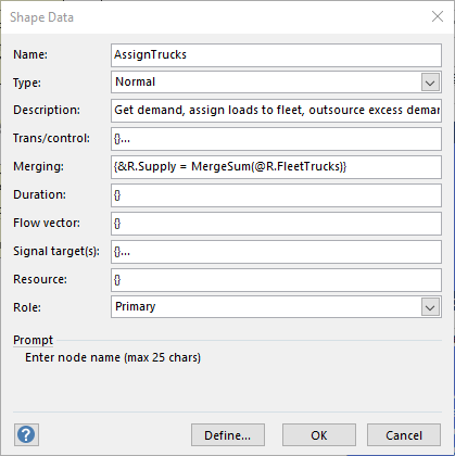
n[5]AssignTrucks: This node fetches demands for each route zone from the Excel table shown earlier in this document, calculates available fleet trucks and determines what loads, if any, should be outsourced. It then creates a temporal connection to a[7] and sends to it different signal entities (calculation threads) carrying fleet truck dispatches to all route zones. Notice in the image of the dialog box below for a[7] that its Branch property is set to No/False. This logical blockage is necessary to ensure that traversal along a[7] is restricted to signals sent from n[5] through the temporal connection. The loads assignment algorithm in n[5] determines how many fleet trucks are dispatched to each route zone. Each signal has properties that carry its assigned route zone and associated number of trucks assigned to the zone. 

a[7]AssignTrucks-->>|AssignTrucks

Signals turn into regular entities when they reach a[7]. NMOD figures out the length of time each entity should take to traverse [7] to get back to n[5] based on the expression you can see in the Duration property box of [7] at left. The value comes from the 8th row of the TruckLdDemand table (shown at top of this page). The column value defining the cell in the 8th row is RouteZone. n[5] also dispatches idle trucks count along a[8] back to itself for the next trucks assignment cycle. Notice that arcs [7], [8], and [4] terminating in n[5] are AND arcs. But, notice also that we have an AND-arc multiplier on [7] (see last element in the Flow vector property). It specifies that entities equaling the number of route zones in the model (tnyMaxZones) must reach n[5] along with the ones arriving through [4] and [8] before [5] can be triggered to start the next cycle.

n[1]Initializations: When the model starts running, all trucks in the fleet are in idle state. This node starts the flow of trucks. n[5]AssignTrucks has AND arcs leading into it, which means that it is a Convergence node requiring arrival of a certain number of entities along those AND arcs before it can be evoked. n[1] needs to supply those entities at the start so that fleet flow can begin.

n[1] has a trigger arc [6] going n[2]DayTracker. An entity launched in this direction will reach n[5] along AND arc [4]. To trigger [5] for the first time, we need 4 more entities to arrive at that node along AND arcs. To accomplish this we first send a signal to a[8] from the SignalTarget property of n[1] in the NET file. The rest of the logic for creating a steady flow of trucks every day into n[5] from all zones is described in the NET file in the properties block for Object 5.

[9]OutsourcingCalcs: This node will be triggered only during the statistics and cost calculation period defined by the analyst. We have defined it to be days 8 through 14. This node tracks how many runs to each zone are outsourced and consequential cost of outsourcing per week.

[14]FleetCalcs: This node will be triggered only during the statistics and cost calculation period defined by the analyst. We have defined it to be days 8 through 14. This node tracks how many runs to each zone are made each week by fleet trucks.

[11]FinalCalcs: This node wraps up results reporting on the final day of the analysis horizon, writing to the Results file certain interesting summary information captured during a model run and all of the calculated costs information.

Fibonacci search procedure in NMOD's Optimization Module was used to find optimal fleet size. Fibonacci search is a procedure for finding optimal value of an integer decision variable (in this case, the number of trucks in the fleet) which produces a unimodal response curve over a decision range. In other words, it was obvious in this case that the total cost curve would go down for a while as the fleet size increases from zero and then at some point would start to go up for larger fleet sizes. Thus, the fleet size that yields the lowest total cost value would be the ideal fleet size.

Using Fibonacci search in a model involves inserting two lines of code in the model, one for providing a stimulus for probing the model and the other for sending the model's response to the optimizer. These lines can remain in the model even if the analyst wants to do just one what-if probe at a time.

The stimulus line should go where the model sets the decision variable's value. In the case of this model, it is in n[1]Initializations. You can locate the stimulus line in the NET file in the 3rd section of n[1]'s Trans property. Look for CALL OptimizationStimulus. This call updates the value of FleetSize with the stimulus value provided by the optimizer. If the model is being run in the what-if probe mode instead, this call will leave FleetSize unaffected.

The response line should go where total costs are computed. You can locate this at the bottom of the Trans property of n[11]FinalCalcs. Look for CALL OptimizationResponse.

• Results from optimization run. You will see how the Fibonacci search figures out that 66 is the optimal fleet size in the search range suggested (50 to 70 trucks), with zero error tolerance, in 6 probes of the model. Since the search called the model 6 times, you will see in the results file 6 executions of the model for different fleet sizes.
  
  If the search range suggested were 0-100 trucks, Fibonacci search would have found the answers with 10 probes. As the suggested search range increases, the economics of this non-naive search procedure becomes exponentially superior to naive searches, such as trivial looping through the search range (shown next).
  
  Since this is a systematic, non-naive search, you will notice from the execution feedback to the screen that the optimizer knows before the search begins how many probes of the model will be necessary to find the optimal answer within the range and the tolerance specified by the analyst.
  
  You can see feedback to the screen from the execution by clicking here.
  
  
• Results from NMOD's Trivial Search procedure. This file contains 21 probes of the model (fleet sizes of 50 to 70), which the stakeholders will be curious to see after they see results from the Fibonacci search. You can see total costs going down until fleet size reaches 66 and starting to increase thereafter. This procedure tracks minimum and maximum values in a range and displays both stimulus-response pairs at the end of the search.
  
  You can see feedback to the screen from this execution by clicking here.
  
  
• Results from a single what-if probe. This was was run by simply changing the Optimization mode in the Excel spreadsheet to 0 and executing the model. We used fleet size of 64 for this exercise.
  
  You can see feedback to the screen from this execution by clicking here.

There are, of course, less naive approaches than the trivial search described above. One approach would be to stop the search immediately, as it proceeds from one end of the solution range to another, when total costs start going up. This too can be cumbersome and inconsistent for large scale models in large ranges. For example, if the range we guessed is 65 to 200, we would have gotten lucky and found the answer in 3 probes. But, if we guessed 0 to 135 instead (same width of range), it would have taken 68 probes to find the optimum.

Downloads of all examples are available in Chapter 1 of the Hands-on Tutorial. However, you can also view all of the examples and their results online without downloading anything.

If you wish to change inputs and execute these models on your PC, or modify them in someway, you will have to NETrans them and create their EXEcutables. To do that you will need to download and install ORMSware and its support components, all of which are available for free trial. Instructions for all of that are available at the above link as well.